Getting Started
Blueprint User Interface
The Blueprint User Interface
The Explorer
The Main Content Area
The Utility Panel
UX Changes in Blueprint 12.2
UX Changes in Blueprint 12.3
Discussions Dashboard
Jobs
Open a Project
Close a Project
Change Your Password
Organize Artifacts and Assets
Status Indicators
Blueprint Help
Search for Help Content
Access the Jobs List
About the Jobs List
Generate Test Cases
About Test Case Documents
Blueprint Release Notes
GenAI
GenAI - Overview
Importing Using GenAI
GenAI Configuration
Create your AI Project
GenAI Import Your First Document
GenAI What's Next
Artifacts
Base Artifacts
Base Artifact Types
Actors
Document Artifacts
Folders
Model Artifacts
Process Artifacts
Textual Requirement Artifacts
User Stories
Reuse, Merge, and Quick Reconciliation
About Reuse, Merge, and Quick Reconciliation
Reuse a Single Artifact
Reuse Multiple Artifacts
Suspect Traces
Merge Artifacts
Quickly Reconcile Artifacts
Descendants View
Using Descendants View
Manage Columns in Descendants View
Filter Columns in Descendants View
Edit Inline in Descendants View
Bulk Edit in Descendants View
Add Artifact Descendants to a Collection, Baseline, or Review in Descendants View
Delete Artifacts in Descendants View
Save a Default View
View and Edit Artifacts in the Utility Panel
View and Edit Artifacts in the Utility Panel
Edit Artifact Properties
View Relationships and Traces
Add Actor Inherits
Add Files to an Artifact
Discussions and Adding Comments
Intelligent Recommendations
Artifact History
Version Compare
Side by Side Version Compare
Restore an Artifact to a Previous Version
Restore Values or Attributes of an Artifact to a Previous Version
Formatting Shapes and Adjusting Canvas Attributes in the Universal Model Editor
Impact Analysis
About Impact Analysis
Initiate an Impact Analysis
Export an Impact Analysis to Excel
Impact Analysis Interface
Access an Artifact’s Properties and Discussions in an Impact Analysis
Traces
Add Traces
Add Traces in the Utility Panel
Add Traces Using the Manage Traces Button
Add Inline Traces Using a Quick Key
Add an Inline Trace with the Links Menu
Add Bulk Traces
Add a Trace to a Sub-Artifact
Add Bulk Traces to Sub-Artifacts
Edit the Direction of Traces
Delete Traces
Glossary
About Glossary
Add Glossary Terms
Edit Glossary Terms
Glossary References
Add a Trace to a Glossary Reference
Create a New Artifact
Visio Import
Visio Mapping
Word Import
Excel Import
Excel Import FAQ
Excel Update
Search for Artifacts
Save and Publish Artifacts
Move Artifacts
Discard and Delete Artifacts
Copy Artifacts
Generate a Document
Steal a Lock
Global Actions
Edit Artifacts in the Process Editor View
Export Artifacts to Excel
Export Artifacts to Word or PDF
Work with Multiple Artifacts Simultaneously
Change an Artifact Type
Visio Import Known Issues
Using a Designated Approval Property
Universal Model Editor
Format Shapes in the Universal Model Editor
Connect Shapes in the Universal Model Editor
Rotate Shapes in the Universal Model Editor
Resize Shapes in the Universal Model Editor
Format Multiple Shapes in the Universal Model Editor
Customize Shapes
Use Shape Commands
Align Shapes in the Universal Model Editor
Shape Reference Guide
Default Library
Basic Library
BPMN Library
Use Case Library
Flow Chart Library
Entity Relationship Library
UI Mockup Library
About the Universal Model Editor
Create a Model Artifact
Customize the Canvas in the Universal Model Editor
Add and Label Shapes to the Canvas in the Universal Model Editor
Move Shapes in the Universal Model Editor
Add Links and Inline Traces to Shapes in the Universal Model Editor
Add and Label Connectors in the Universal Model Editor
Container Shapes in the Universal Model Editor
Pool Shapes
BPMN Variations in the Universal Model Editor
Shapes as Sub-Artifacts
Print Model Artifacts
Convert Legacy Blueprint Diagrams
Collections
About Collections
Create a Collection
Add Artifacts to a Collection
Remove Artifacts from a Collection
Manage Columns in a Collection
Filter Columns in a Collection
Bulk Edit in Collections
Edit Inline in Collections
View and Edit Collection Artifacts in the Utility Panel
Add Collection Artifacts to a Baseline or Review
Export Artifacts to Excel in Collections
Export Collection Artifacts to Word or PDF
Baselines
About Baselines
Create a Baseline
Add Artifacts to a Baseline
Remove Artifacts from a Baseline
Set a Timestamp in a Baseline
Seal a Baseline
Reviews
Participate in Reviews
About the Review Experience
The Review Experience User Interface
The Review Experience Utility Panel
View and Approve Artifacts in a Review
Filter Your Review in the Review Experience
Discussions and Adding Comments in the Review Experience
Display Only Descriptions and Diagrams in a Review
Track Your Review Progress in the Review Experience
Complete a Review in the Review Experience
Manage Reviews
Create a Review
Add Artifacts to a Review
Add Unauthorized Artifacts to a Review
Remove Artifacts from a Review
Set the Approval Status for a Review
Add Participants to a Review
Remove Participants from a Review
Set Roles for a Review
Add Instructions to a Review
Start a Review
Manage Discussions in a Review
Require Participants to Complete a Full Review
Require Review Approvals to Have Electronic Signature
Add an Electronic Signature and Meaning of Signature to a Review
Set an Expiration Date for a Review
Monitor and Analyze Statistics in a Review
View Artifacts' Individual Metrics and Details Reports in a Review
Close a Review
Create a Follow-up Review
Review Notifications
Configure Review Notifications
Add and Assign Meaning of Signature
About Reviews
Types of Reviews
Workflows
Workflow Canvas
About the Workflow Canvas
The Workflow Canvas vs Workflow XML Definitions
Create and Define a Workflow with the Canvas
Define Actions in a Workflow that are Triggered by Transitions
Workflow XML-Canvas Interaction
Workflow XML Examples and Reference
Transitions as Triggers Workflow Example
Linear Progression Workflow Example
Loopback Workflow Example
Branching Workflow Example
Trigger and Action Examples
Artifact Creation and Property Update Triggers Workflow Example
Associate Workflows with Artifact Types and Projects Example
Workflow XML Reference
Workflow XML Reference - Action Properties
Workflow XML Reference - Triggering Events and Parameters
Workflow XML Reference - Triggering Events and Valid Actions
About Workflows
Workflow Components
Put Workflow Components Together
Create a Workflow
Edit a Workflow
Delete a Workflow
Disable a Workflow
Upload a Workflow
Download a Workflow
Copy a Workflow
Use Webhooks with a Workflow
Using Legacy Blueprint When a Workflow is Enabled
Administration
System Reports
System Reports
License and Activity Reporting
User List
Project Activity
User Roles
Artifact Map
Project Usage
User Activity Report
Audit Log
Download User Logs
User Management
Federated Authentication
About Federated Authentication
About Fallback from Federated Authentication
Active Directory and Federated Authentication Settings
Configuring your Identity Provider for Blueprint Federated Authentication
Enabling Blueprint Federated Authentication
Managing Active Directory Settings
Configuring Default Active Directory Integration
Configuring Custom Active Directory Integration
Disabling Active Directory Settings
Create New Users
Edit Users
Delete Users
About Groups
Create New Groups
Add Users to Groups
Edit Groups
Delete Groups
About Project Groups
Manage Project Groups
Add a Project Group
Edit a Project Group
Copy a Project Group
Delete a Project Group
Delete Multiple Project Groups
Assign Members to a Project Group
Unassign Members from a Project Group
Assign Project Roles to a Project Group
Select the Scope of Project Role Assignments on a Project Group
Unassign Project Roles from a Project Group
Project Role Assignments
Add New Role Assignments
Edit Role Assignments
Delete Role Assignments
About Project Roles
Manage Project Roles
Add a Project Role
Edit a Project Role
Copy a Project Role
Delete a Project Role
Delete Multiple Project Roles
Assign Project Groups to a Project Role
Unassign Project Groups from a Project Role
Select the Scope of Project Group Assignments on a Project Role
Instance Administrator Roles and License Types
Manage Instance Administrator Roles
Instance Administrator Role Privileges
Create an Instance Administrator Role
Edit an Instance Administrator Role
Copy an Instance Administrator Role
Delete an Instance Administrator Role
Delete Multiple Instance Administrator Roles
Assign Users to an Instance Administrator Role
Unassign Users from an Instance Administration Role
Integration Role
Project Administrator Roles and Privileges
Manage Project Administrator Roles
Create a Project Administration Role
Edit a Project Administrator Role
Copy a Project Administrator Role
Delete a Project Administrator Role
Delete Multiple Project Administrator Roles
Send New Users a Welcome Email
Project Management
Create a New Folder in a Project
Edit Folders
Delete Folders
Create a New Project
Edit Projects
Delete Projects
About Project Artifact Types
Manage Project Artifact Types
Add a Custom Artifact Type
Edit a Project Artifact Type
Copy a Project Artifact Type
Assign Project Properties to a Project Artifact Type
Unassign Project Properties from a Project Artifact Type
Manage Sub-Artifact Types
Delete a Custom Artifact Type
Delete Multiple Custom Artifact Types
Enable a Standard Artifact Type in a Project
Disable a Standard Artifact Type in a Project
About Project Properties
Manage Project Properties
Add a Custom Property
Edit a Custom Property
Copy a Project Property
Add Valid Values to a Choice Type Custom Property
Edit Valid Values for a Choice Type Custom Property
Delete Valid Values from a Choice Type Custom Property
Delete a Custom Property
Delete Multiple Custom Properties
About Project Templates
Add Project-Level Office Document Templates
Edit Project-level Office Document Templates
Add User Inputs to Project-level Office Document Templates
Edit User Inputs to Project-level Office Document Templates
Delete User Inputs for Project-level Office Document Templates
Copy Project-level Office Document Templates
Delete a Project-level Office Document Template
Delete Multiple Project-Level Office Document Templates
Set or Reset a Project Print Template
Download a Project Print Template
Import and Export Projects
Instance Administration
About Standard Artifact Types
Manage Standard Artifact Types
Add a Standard Artifact Type
Edit a Standard Artifact Type
Copy a Standard Artifact Type
Assign Standard Properties to a Standard Artifact Type
Unassign Standard Properties from a Standard Artifact Type
Assign Projects to a Standard Artifact Type
Unassign Projects from a Standard Artifact Type
Manage Reuse Settings for Standard Artifact Types
Delete a Standard Artifact Type
Delete Multiple Standard Artifact Types
About Standard Properties
Manage Standard Properties
Add a Standard Property
Edit a Standard Property
Copy a Standard Property
Add Valid Values to a Choice Type Standard Property
Edit Valid Values for a Choice Type Standard Property
Delete Valid Values from a Choice Type Standard Property
Delete a Standard Property
Delete Multiple Standard Properties
Instance Settings
Define Access and Logging In Settings
Instance Security Settings
Define Import and Export Settings
Define Bulk Edit Settings
Define File Upload Restrictions Settings
Define Attachments Settings
Define Trace and Reuse Settings
Define Move and Copy Settings
Define Rich Text Settings
Define Process Settings
Define Models Settings
Email Settings
Configure Email Credentials
Configure Your Incoming Mail Server
Configure Your Outgoing Mail Server
Configure Email Notifications
Templates
Add Office Document Templates
Edit Office Document Templates
Add User Inputs to Office Document Templates
Edit User Inputs for Office Document Templates
Delete User Inputs for Office Document Templates
Copy Office Document Templates
Delete Office Document Templates
Set or Reset an Instance Print Template
Download an Instance Print Template
External URLs
Configuring a Designated Approval Property
About the Administration Portal
Instance Administration Guide
Project Administration Guide
Analytics User Guide
Blueprint Installation Guide
System Requirements
Supported Third-Party Components
Supported ALM Integrations
Digital Blueprint Licensing in Blueprint
Artifact Author as Default Value
Federated Authentication Settings
Process Editor
User Stories
About User Stories
Generate User Stories
Generated User Story Components
User Story Artifacts
Initiate a User Story Walkthrough
Preview User Stories
Link User Stories to Other Artifacts
Download User Story Work Items
About the Process Editor
Create a Process Artifact
Enable System Steps
Model a Process
Add and Label a Task in a Process
Add and Label Conditions in a Process
Add and Label Choices in a Process
Add and Label a System Task in a Process
Add Multiple System Steps in a Process
Delete Choices and Conditions in a Process
Move Tasks in a Process
Copy and Insert Tasks in a Process
Add Details to Tasks and Decision Points in a Process
Efficiently Add Screenshots
Define a System Actor and System Response
Add an Image to Support a System Response
Add and Modify Choice and Condition Endpoints
Include Other Processes within a Process
Include Another Process or Artifact Within a Process
View a Process in Text View
Moving From Use Cases to Processes
Compare to Latest Version
Digital Blueprints
Intelligent Process Conversion
Working with Large Processes
Blueprint REST API
REST API Requests
REST API - Authenticate Request
REST API - List Projects Request
REST API - Get Project by Id Request
REST API - Create Project Request
REST API - List Artifacts Request
REST API - Get Artifact Request
REST API - Get Child Artifacts of Artifact Request
REST API - Get Root Artifacts of Project Request
REST API - Add Artifact Request
REST API - Update Artifacts Request
REST API - Delete Artifact Request
REST API - Publish Artifact Request
REST API - Discard Artifacts Request
REST API - List Unpublished Artifacts Request
REST API - Get Collection Request
REST API - List Collections Request
REST API - Get Attachment Request
REST API - Add Attachment Request
REST API - Add Attachment to Subartifact Request
REST API - Delete Attachment Request
REST API - List Groups Request
REST API - Get Group Request
REST API - Add Traces Request
REST API - Move Artifact Request
REST API - Delete Traces Request
REST API - List Users Request
REST API - Get User Request
REST API - Create User Request
REST API - Update User Request
REST API - Delete User Request
REST API - List Artifact Types Request
REST API - Get Artifact Type Request
REST API - Get Discussion Status Request
REST API - Update Standard Choice Property Request
REST API - Update Custom Choice-Property Type Request
REST API - Add Comment Request
REST API - Rate Comment Request
REST API - Publish Comments Request
REST API - Update Comment Request
REST API - Delete Comment Request
REST API - Reply to Comment Request
REST API - Rate Reply Request
REST API - Update Reply Request
REST API - Delete Reply Request
REST API - Get Artifact Image Request
REST API - Get Blueprint Product Version Request
REST API - List Reviews Request
REST API - Get Review Request
REST API - Close Review Request
REST API - Import Task Capture Payload
REST API - Get Information of Import Task Capture Payload Job Request
REST API - Get Information of Import Task Capture Payload Jobs Request
REST API Request Body and Parameters
REST API - Filter Parameter
REST API - Listing Artifacts in the Request Body
REST API - Defining an Artifact in the Request Body
REST API - Defining a Trace in the Request Body
REST API - Defining a User in the Request Body
REST API - Defining a Comment in the Request Body
REST API - Defining a Reply in the Request Body
REST API - Defining an ALM Job in the Request Body
REST API Request Header and Parameters
REST API HTTP Methods
REST API - HTTP HEAD Method
REST API - HTTP GET Method
REST API - HTTP POST Method
REST API - HTTP PATCH Method
REST API - HTTP DELETE Method
Blueprint REST API
REST API Requests
REST API Security and Authentication
REST API Requests and Responses
REST API HTTP Status Codes
REST API Resources
REST API Quick Start Example
REST API Known Issues & Constraints
Document Template Authoring
Document Template Authoring Tutorial
Getting Started with Office Document Template Authoring Tutorial
Install the Blueprint Template Authoring Add-in for Microsoft
Download and Open a Sample Template
Download your Blueprint Project XML Data and Add it as a Data Source
Customize and Test the Document Template
Add the Document Template to Blueprint
Document Template Data Sources
About Data Sources
Add and Connect to a Data Source
Edit a Data Source Connection
Delete a Data Source Connection
Document Templates and Pods
Document Template Authoring and Tags
About Tags
Tag Tree
Tag Editor
If Tag
If Tag Tutorial
Else Tag
Else Tag Tutorial
ForEach Tag
ForEach Tag Tutorial
Import Tag
Import Tag Tutorial
Link Tag
Link Tag Tutorial
Out Tag
Query Tag
Query Tag Tutorial
Set Tag
Switch Tag
Add Tags in Excel
Add Tags with the Data Bin
Add Tags with the Data Tree
Add Tags with the Tag Builder
Insert Tags within a ForEach Tag
Edit Tags in your Document Template
Delete Tags in your Document Template
Evaluate Tags
Validate Tags
Document Template Variables
Document Templates and Equations
Author Document Templates
About Generating Output
AutoTag Output Formats
Generate a Document with the Add-in
Generate a Document that Contains a Variable with the Add-in
Document Template Options and Parameters
XPath Selects
The XPath Wizard
Sort XML Datasources
Conditional Formatting for Document Templates
Create Dynamic Formulas in Microsoft Excel
Embedded Objects
Event Handler
HTML Fragments
Tools
Blueprint for Enterprise Agile Planning
Blueprint 12.2 UI Updates
Model Artifacts vs Process Artifacts
Process Decomposition
Process artifact: Generate Tests & Feature Files
Tracing Overview
Tracing Methodology - Direction of Traces
Ordering User Stories (and artifacts)
Manage User Stories
How to use Collections
Baselines and Reviews
Use Case conversion to Process Artifacts
Import; Word, Excel, and Visio
Reuse Library Example
- All Categories
- Document Template Authoring
- Create Dynamic Formulas in Microsoft Excel
Create Dynamic Formulas in Microsoft Excel
How to take advantage of Microsoft Excel's dynamic formulas – formulas that produce data on the fly – in Blueprint document templates.
You can take advantage of Microsoft Excel's dynamic formulas – formulas that produce data on the fly – in Blueprint document templates. AutoTag carries functions across cells, and it knows when to include new cells and when to change range numbers. Here we will walk though two simple examples while keeping in mind that AutoTag has much more sophisticated dynamic formula capabilities.
This tutorial begins with a blank template connected to the Northwind XML data source. For more information on how to connect to a data source, see the Data Sourcing article.
Tutorial
Step 1 - Create a Table
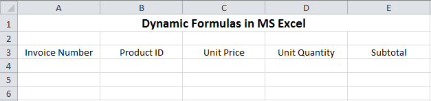
Before you can begin placing tags in the template, you need to know where they will go. In this example, you will be creating a table of products and information about those products.
This table will have columns for the invoice number, the product ID, the product's unit price, the product's quantity, and a column subtotalling the cost of each product ordered.
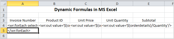
Choose ten cells in Excel in which you will create a 5 by 2 table. This size is chosen because it provides one column for each data category. In the first row, place the data titles, and in the second row, place the tags.
You do not need to know how many rows of data will be output when you run the report; AutoTag takes care of expanding that for you automatically.
In the table's first row, enter the column headings:
Step 2 - Create a <forEach> Tag
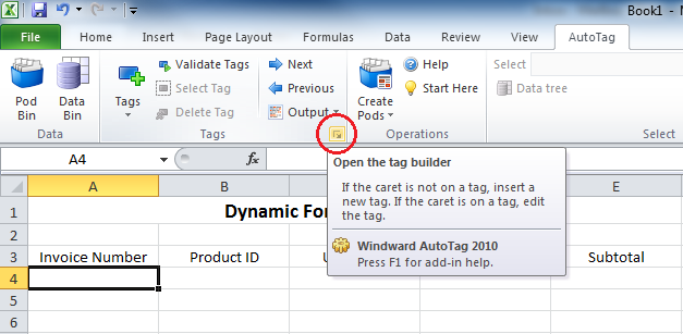
- Click the first cell in what will be the second row of the table (the cell A4 in the image above).
- Click the Tag Builder button.
- In the Tag Editor, click the Tags tab, and click the <ForEach> Tag icon.
- Click the Select tab. Since you will be creating a table of data from subgroups of the Order Details data group, that's the group you want to loop through.
Click the Order Details data group in the Data Source pane, and drag and drop that group into the Select Bar. - Give the variable a descriptive name, such as "orderdetails." The tag editor now looks like this:
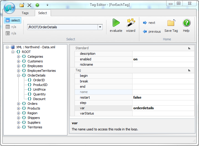
- Save the tag.
Step 3 - Create the First <out> Tag
Now it's time to place data subgroups into the individual cells.
Click the cell that holds the <forEach> tag, and click the Tag Builder button. A prompt appears, asking you where you'd like to place the tag:

Place your cursor just after the colon (:) and click.
The Tag Builder window opens. Follow the same general procedure as you did with the <ForEach> tag, with a few changes:
- Click the Tags tab and click the <Out> Tag icon.The <out> tag is the default tag type, so this is already done for you
- Click the Select tab.
- In the Data Source pane, click the + sign next to the <forEach> tag name that you created – in this case, orderdetails – to expand it.
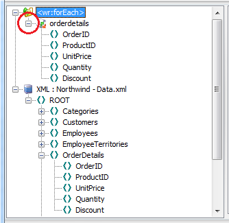
- The OrderID group contains the invoice number, so drag the OrderID data subgroup from the orderdetails variable into the Select Bar.Be sure to drag and drop the correct OrderID data subgroup, as there are two listed in the Data Source Pane.Drag and drop the data subgroup from the orderdetails variable, not from the main data source listed below it.
- Save the tag.
Step 4 - Create Additional <out> Tags
Using the same procedures that you followed in step three, create <out> tags for the three remaining cells.
The ProductID subgroup goes in the select bar for the tag in the Product ID column, the UnitPrice subgroup goes in the select bar of the tag in the Unit Price column, and the Quantity subgroup goes in the select bar of the tag in the Unit Quantity column.
Of course, each of these <out> tags will be in its own cell, so you will not see a prompt asking you where to insert the tag.
Step 5 - Close the <forEach> Loop
Next is to place data subgroups into the individual cells.
Click the cell that holds the <forEach> tag, and click the Tag Builder button. A prompt appears, asking you where you'd like to place the tag:
Step 6 - Create a Dynamic Formula for Multiplication
In the first example, we want to know how much is being spent on each item. In other words, we want to multiply the unit price by the unit quantity for each item, and that will give us our subtotal.
Click the cell below the cell labeled "subtotal."
Enter the formula Excel uses for multiplication, which is an equals sign, the location of the first cell to be multiplied, an asterisk, and the location of the second cell to be multiplied. Your template should resemble the following:
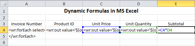
The power in using this formula is that AutoTag automatically expands the Subtotal cells to match the data. Instead of one subtotal, you will see a subtotal for each row. The database contains hundreds of orders, but you only have to input the formula once.
It's unlikely you will name a macro with 1 or 2 letters followed by a number. But if you do, AutoTag breaks because it will change the macro if it’s moved/replicated in the final report.
Step 7 (Optional) - Filter the Table
It is not necessary to add filters to our table in order to demonstrate formula features in Excel, but because you are working with a large set of data, you will do so now for two reasons: Your data source is quite large, and this will make illustrating the next formula much simpler.
Plus, the formula you are going to create will sum items, and using a filter now will allow you to demonstrate a very practical application: summing items and coming up with a total cost for a particular invoice in your system.
To begin:
- Click the cell containing the <forEach> tag and click the Tag Editor button.
- In the prompt, click the <forEach> tag.
- In the Tag Editor, click the Wizard icon.
What you do next will depend upon the data source you're using, because the wizards are different for XML and SQL data sources.
XML Data Source
- In the Conditions Pane (the left pane), click the statement [click here to add a group]
- Click the statement [click here to enter a condition]
- Click the statement [click here to select a node], and select the subnode (subgroup) OrderID. (Remember, OrderID is the invoice number.)
- By default, the comparison is set to equal to, so you do not need to select a comparison.
- Take a look at the various OrderID values listed in the Data Pane on the right. There's one for invoice number 10248, and that's the one we'll use in our example. Click the statement [click here to set the value] and in the text box, enter the number 10248.
- You can see the entire select statement (the query that will be sent to the data source when you run the report) in the lower pane of the wizard. Click OK. This closes the XPath Wizard.
- Click the Save Tag icon. Your <forEach> tag (as seen in the formula bar) now looks like this:

SQL Database
- Drag the desired node (in this case, Order Details) from the left pane into the Columns area of the middle pane.
- In the Filter area of the middle pane, click the statement [click here to add a group]
- Click the statement [click here to add a filter]
- Click the statement [click here to select a node], and select the subnode OrderID from the pop-up window. (Remember, OrderID is the invoice number.)
- By default, the comparison is set to equal to, so you do not need to select a comparison.
- Take a look at the various OrderID values listed in the Data Pane on the right. There's one for invoice number 10248, and that's the one we'll use in our example. Click the statement [click here to set the value] and in the text box, enter the number 10248.
- You can see the entire select statement (the query that will be sent to the data source when you run the report) in the lower pane of the wizard. Click OK to close the wizard.
- Click the Save Tag icon. The end of your <forEach> tag (as seen in the formula bar) now looks like this:

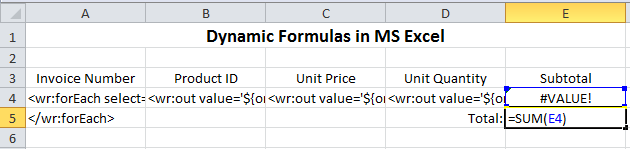
Step 8 - Create a Dynamic Formula Using Excel's Autosum Feature
Now it's time to place data subgroups into the individual cells. Click the cell that holds the <forEach> tag, and click the Tag Builder button. A prompt appears, asking you where you'd like to place the tag:
From Excel's Home tab, click the AutoSum icon. In the formula =SUM() put the location of the subtotal value, which in our example is E4, between the parentheses. Your template now looks like this:
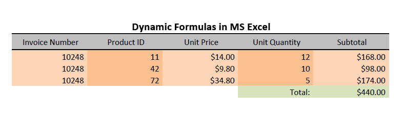
Step 9 - Format the Table
Use familiar Excel commands, such as those in Excel's Home menu, to clean up the table. Because columns C and E are currency, format the columns accordingly. Also, change the font, add colors, reposition text, place borders around cells, and otherwise enhance the look of the table.
Save your document template using Excel's Save command. Then, from the AutoTag Run Report group, click the desired report format icon. In this example, we chose to view the report as a PDF file, and this is the result:
You may need to tweak your table dimensions a bit, as Excel does not let you auto-expand a cell as needed.
How did we do?
Conditional Formatting for Document Templates
Embedded Objects